想设计一个公司的网站网络营销的现状

固体比热模型中的德拜模型和爱因斯坦模型是固体物理学中用于估算固体热容的两种重要原子振动模型。

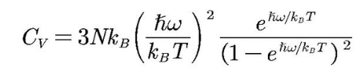
爱因斯坦模型基于三种假设：1.晶格中的每一个原子都是三维量子谐振子；2.原子不互相作用；3.所有的原子都以相同的频率振动（与德拜模型不同）。

在高温下，爱因斯坦模型与实验结果一致，特别是与杜隆-珀替定律相符‌。

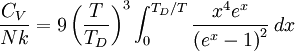
德拜模型将晶体中的原子振动视为连续弹性介质中传播的弹性波。固体的热容主要由低频的声学支声子贡献，存在截止频率，并未考虑光学支声子的贡献。在低温区与实验结果高度一致。

基本设置

import numpy as npimport osimport matplotlib.pyplot as pltfrom scipy.optimize import curve_fitimport scipy.integrate as integrate
from scipy.integrate import quad
R = 8.3144  # unit: J/ (mol·K）N = 10   #number of atomsn = 0.5 #Debye/(Debye+Einstein)names = ["data.dat"]colors = 'rgbmpyckrgbmpyc'

数据读入

def readata(name):    try:        data = np.loadtxt(name)          T = data[:, 0]        T = np.flipud(T)        HC = data[:, 1]  # HC        HC = np.flipud(HC)        #print(f"Data read from {name}:")        #print("T:", T)        #print("HC:", HC)        return T, HC    except ValueError:        print('empty value encountered in', name)        return None, None

德拜模型

    def intdebye(x):        return x**4 * np.exp(x) / (np.exp(x) - 1)**2       HC_calc_debye = []        for Ti in T:        A1 = quad(intdebye, 0, ThetaD / Ti)[0]          debye_value = 9 * R * N * (Ti / ThetaD)**3 * A1        HC_calc_debye.append(debye_value)    HC_calc_debye = np.array(HC_calc_debye)

爱因斯坦模型

    HC_calc_Einstein = []       for Ti in T:        einstein_value = 3 * R * N * (ThetaE / Ti)**2 * np.exp(ThetaE / Ti) / (np.exp(ThetaE / Ti) - 1)**2        HC_calc_Einstein.append(einstein_value)    HC_calc_Einstein = np.array(HC_calc_Einstein)

HC模型混合（将D和E模型填入）

def HC_lattice(T, ThetaD, ThetaE):    HC_lattice = n * HC_calc_debye + (1 - n) * HC_calc_Einstein        return HC_lattice    

磁熵或相变熵值计算和统计

def S_CT(T, C_mag):    CoT = C_mag / T    S = np.cumsum(CoT)    #print("S:", S)    return S    S_integral = integrate_S(T, S, 0, 50)    #print(f'n={n:.1f}, S_integral from 0 to 50: {S_integral:.3f}')    print("S:", S_integral)    return S_integral

拟合区间函数设定

def FitRange(lower, upper, numbers):    ii = np.argmin(np.abs(numbers - lower))    jj = np.argmin(np.abs(numbers - upper))    return min(ii, jj), max(ii, jj)    #lower, upper = FitRange(25, 200, T)  # claim the lower and upper range of fitting    #popt, pcov = curve_fit(HC_lattice, T[lower:upper], HC[lower:upper])   

读入数据拟合和绘图

for i, name in enumerate(names):    print(name)    T, HC = readata(name)        if T is not None and HC is not None:        if 'data' in name:            color = colors[i]            plt.subplot(2,2,1)            plt.plot(T, HC, color + 'o', label=name)            plt.xlabel('T(K)')            plt.ylabel('HC(J/K/mol)')            plt.legend()                        lower, upper = FitRange(25, 200, T)  # claim the lower and upper range of fitting            popt, pcov = curve_fit(HC_lattice, T[lower:upper], HC[lower:upper])                        ThetaD,ThetaE=popt            print('fit:  ThetaD=%5.3f, ThetaE=%5.3f' % (ThetaD,ThetaE))            plt.subplot(2,2,2)            plt.plot(T, HC_lattice(T, *popt), 'k-', label="HC_lattice")            plt.plot(T, HC, color + '*', label="HC_exp")            plt.xlabel('T(K)')            plt.ylabel(r'$HC(J/K/mol)$')            plt.legend()                        C_mag = HC - HC_lattice(T, *popt)            plt.subplot(2,2,3)            plt.plot(T, C_mag, 'k*', label="C_mag")            plt.plot(T, HC, color + '*')            plt.xlabel('T(K)')            plt.ylabel(r'$HC_mag(J/K/mol)$')            plt.legend()                                                plt.subplot(2,2,4)                        S_mag = S_CT(T[1:], C_mag[1:])            plt.plot(T[1:], S_mag, 'k-', label="S_mag")            plt.plot([0, 300], [R * np.log(2 * 5 / 2 + 1), R * np.log(2 * 5 / 2 + 1)], 'r-', label="S=5/2")            plt.plot([0, 300], [R * np.log(2 * 4 / 2 + 1), R * np.log(2 * 4 / 2 + 1)], 'b-', label="S=2")            plt.plot([0, 300], [R * np.log(2 * 4 / 4 + 1), R * np.log(2 * 4 / 4 + 1)], 'm-', label="S=1")            plt.legend()
plt.show()#plt.savefig("1.png")